gene_analysis and can be used to find peaks in histograms and match them across different samples.
Its output is either an MxN similarity matrix of zeros and ones that mark the coinciding peaks,
where M is the number of samples and N is the number of bins in the histogram.
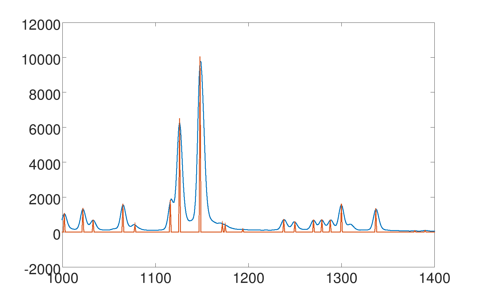
Finding Peaks
First, the program must be compiled. You can use make or do it by hand:
gcc -std=c99 -Wall -o gene_analysis gene_analysis.c -lm
The available parameters to the program can be listed:
gene_analysis -help
At the moment, .fsa files cannot be read directly.
Instead, they must be exported to text files with the GeneMarker program.
The program can then be used in different ways:
In order to find and print all peaks in the data of dye number 2, the program must be called with the following options:
gene_analysis -in TraceData*.txt -print peaks 2 > peaks_yellow.txt
Note: The dyes (e.g. blue, green, yellow) are enumerated, starting with 0, so -print peaks 2 means "print all peaks of the third dye".There are additional possible parameters that have been omitted in this simple example. If a parameter is not given, a reasonable default value is chosen (see help output). The output is redirected to the text file "peaks_yellow.txt". It will have all values set to 0, except the peaks, so it will for example look like:
    0 0 0 0 0 145 0 498 250 ...
    0 0 0 0 0 210 0 0 319 ...
If the parameter -normalize is used, each row is normalized, so the sum of all values is equal to 1.
This is useful if the data is later fed into a machine learning algorithm.
Here is an example, in which almost all parameters are set:
gene_analysis -mov_avg_1 10 -mov_avg_2 100 -bins_ignore_after 350
  -in TraceData_Platte* -min_val 50 -min_diff 20 -print peaks1 2
  > peaks1_yellow.txt
Note: Although the command line is wrapped here, it must be written in one line.
Also note that in this example, -print peaks1 2 is used, which prints a 1 at each position of a peak.
So if the same input data were used as in the example above, the file "peaks1_yellow.txt" would look like this:
    0 0 0 0 0 1 0 1 1 ...
    0 0 0 0 0 1 0 0 1 ...
That is, if with the different parameters for the moving average and the different threshold the same peaks are found.
The parameter -bins_ignore_after is used to only include all bins up to 350.
Note that since the data is upsampled by a factor of 10, the first 3500 entries are actually processed, and the results is later 10x subsampled, resulting in 350 bins.
If the data has been upsampled by a different factor than, it can be specified with the parameter -downsample.
There are also other -print options:
-print data N prints the complete data of dye N.
-print inspect N prints the complete data of dye N.
Similarity Matrix
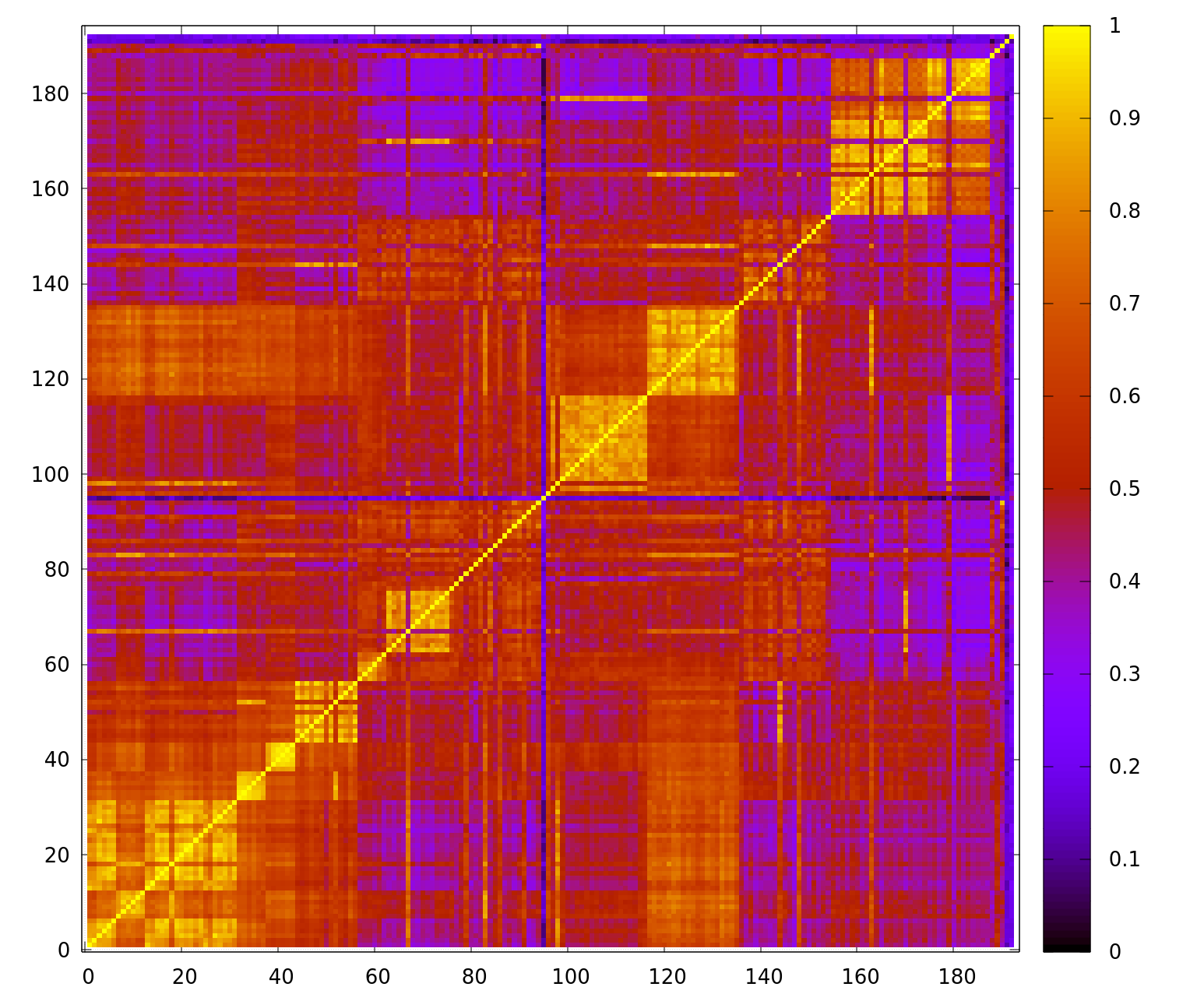
The program can also calculate a similarity matrix of samples by first finding all peaks in all samples and then matching them with the peaks of all other samples. The result is an MxM matrix, where M is the number of samples.
In the following example, the similarity matrix of all samples and the first dye (dye 0) is calculated:
gene_analysis -in TraceData_Platte* -print similarity 0
  > similarity_blue.txt
All parameters that affect the peak finder can also be given, for example:
gene_analysis -in TraceData_Platte* -min_val 100 -min_diff 20
  -print similarity 1 > similarity_greem.txt
Peaks of different samples are sometimes not exactly aligned, but in neighbouring bins, for example:
sample A:    ... 0 0 0 1 0 0 ...
sample B:    ... 0 0 1 0 0 0 ...
When the similarity is calculated, such mismatches can be tolerated and counted as coinciding peaks by passing the -tolerant to the program:
gene_analysis -in TraceData_Platte* -print similarity 0
  -tolerant > similarity_blue.txt
Finally, the similarity matrix can be visualized in gnuplot with the following command:
plot 'similarity_blue.txt' matrix nonuniform with image notitle
Self-Organizing Maps
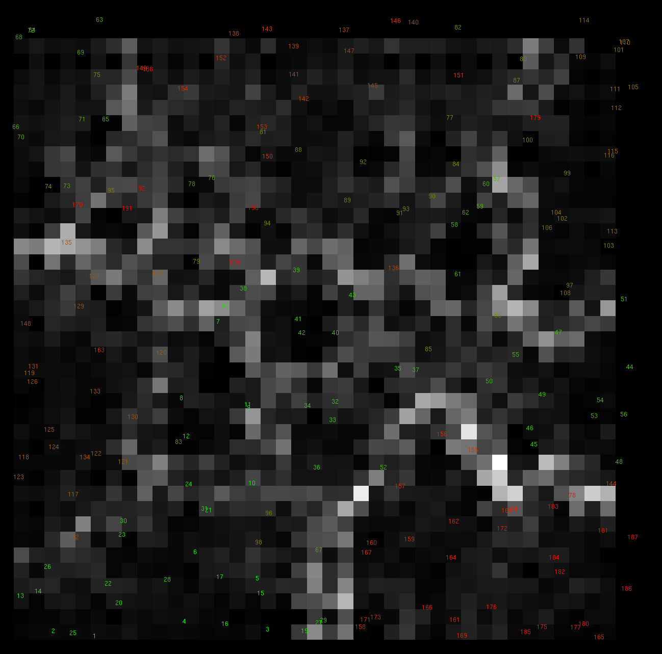
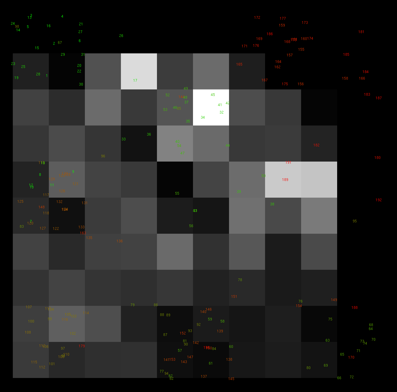
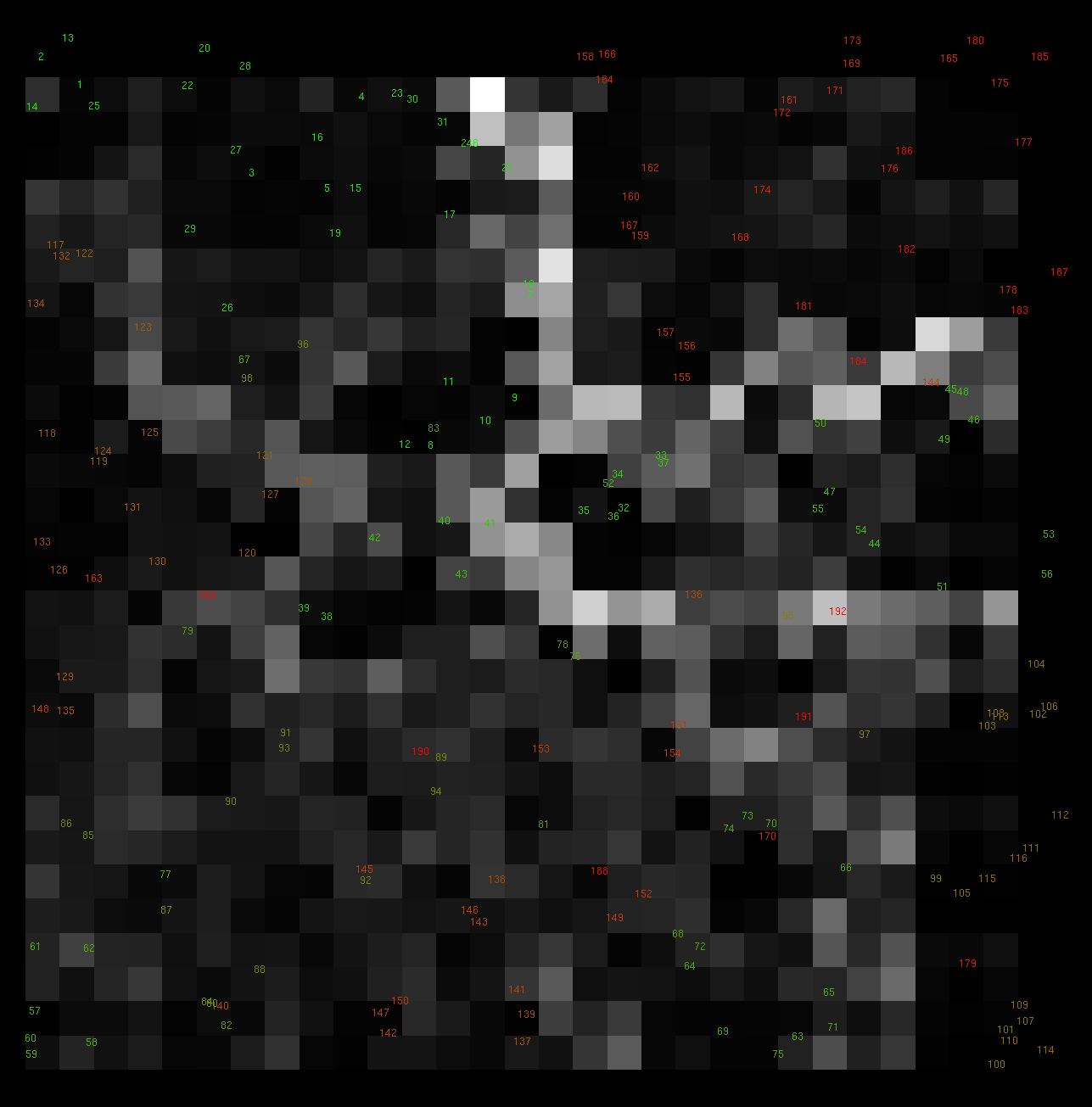
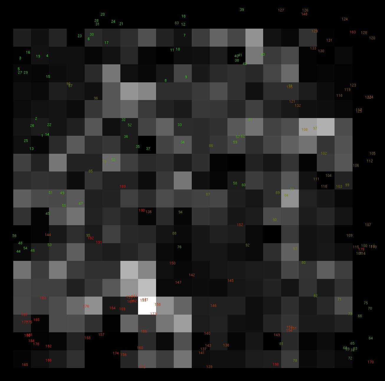
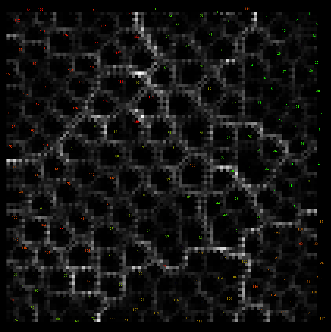
Explanation: ToDo......

